Solar Electric Facility O&M: Now Comes the Hard Part

The omission can be attributed to a pervasive misconception that solar is a static technology: build it and it will work error-free for 30 years. This philosophy works well in a dark vacuum. But in the unpredictable cycles of earthly weather, solar facilities require a watchful eye, intuition, skilled hands and a budget. In a sense, operating a solar array of any size is similar to raising a child. They’re expensive and each one has its own personality requiring patience and considerable attention.

As Director of Asset Management Services for Solar Power Partners, I oversee the health and wellbeing of over 40 solar electric facilities (SEFs) generating more than 21 gigawatt-hours a year. Our principal business is in financing, owning and managing a constellation of commercial-scale SEFs including fixed rooftop arrays, fixed elevated arrays, tracking elevated arrays and single and dual axis ground mount arrays. System sizes range widely from 100kW up to 2.4 MW and our PPA customers include schools, universities, airports, retail stores and municipalities. All told, our portfolio of assets is a cross section of distributed solar.

It is also a daunting exercise in O&M made manageable with accurate upfront performance modeling, a reliable and effective monitoring system, active monitoring by knowledgeable personnel, realistic preventative maintenance policies and budgets, solid warranty backing, efficient reactive repair policies and targeted analytics.

This is the first of three articles that will focus on O&M issues for solar electric facilities. We begin by examining some of the factors that contribute to an effective O&M strategy. In Part II, which will appear in the November/December issue, we will look at preventative maintenance strategies, warranties and budgets. Part III, scheduled for the January/February issue, will look both at critical and non-critical reactive repairs.

Our business works closely with key integrators in the industry and we recognize their expertise in the installation of solar arrays. However, we do place requirements on our partners including the use of best of breed components, specific monitoring equipment and best practices in installation. The purpose is to ensure the longevity and reliability of output from our arrays. This equates to predictability, which is vital to solar financing.

To further strengthen performance predictability, both Solar Power Partners and a third party engineering firm–independent of each other–create projected production models by using historic weather data and by making performance assumptions. These assumptions range from highly predictable (temperature degradation and line losses) to highly unpredictable (soiling and downtime). Interestingly, it is the unpredictable that we have the most control over through O&M. This fact, coupled with an adequate O&M budget, lowers performance risk and improves the financial attractiveness of a SEF to our financial partners. Lower risk results in lower finance costs that more than pay for the cost of O&M.

Competent production estimates benefit not only solar finance efforts; they provide a basis from which to measure system performance through time. With two simple pieces of information (actual monthly output and predicted monthly output) the O&M manager can make elementary inferences to the condition of an SEF. This is a good start, akin to judging a person’s health by the glow of their skin. But healthy skin does not necessarily equate to peak performance. To adequately judge health and performance we need more refined diagnostic tools.

The Monitoring System

Not long ago, the only way to actively monitor an SEF was to compare actual energy production from the meter to predicted energy production. It remains important today due to its simplicity, affordability and reliability. With this simple information an experienced O&M manager can deduce the general health of an SEF; a method sufficient when system optimization is not a top priority. But beyond the few highly incentivized solar regions on earth, production optimization is an urgent concern, not simply to maximize income but to make solar energy financially feasible.

To meet the predicted output of an SEF, we need to ensure that its components function efficiently throughout the system life. This requires a higher degree of granularity than the production meter alone can provide. Luckily, a number of options exist that increase in resolution as we move further from the production meter and closer to the solar energy source.

 

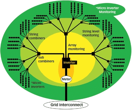
Inverter Monitoring: (Figure 1, above, orange elipse). Most major inverter manufacturers provide a menu-driven user interface imparting access to the inverter’s status, adjustable parameters and historic operating data. This access is vital because the inverter tends to be the lynchpin of any system and the SEF as a whole will only perform up to the operating level of the inverter, never beyond.

The data presented by the inverter tends to be in a format that is both logical and informative. For instance, the inverter will tell us how much DC power is being fed into the inverter, how much AC power is being produced on the back end and how efficiently the power inversion is being performed. It also self-monitors and informs us where problems lie within the inverter, often before they become critical. Because a commercial solar energy system already requires an inverter, the additional costs associated with this method of system monitoring lie in information gathering. If the asset manager is not on site then site visits must be scheduled or a remote Ethernet link established through the inverter’s communications port.

Array Monitoring: (Figure 1, yellow area). This offers a finer degree of resolution and can be simple or complicated depending on the desired level of granularity and the design of the SEF. In principle it involves reading the DC current being produced from sections of the array and relaying that information to the system manager. In its simplest form (not shown) an array designed with many small, monitored inverters provides array monitoring by default because a small section of the array can be monitored through its dedicated inverter. In an array with a large inverter, the simplest solution is to mount DC current transducers (CTs) on the incoming DC homerun cables entering the inverter cabinet. The transducers transmit current flow information from different sections of the array into a data acquisition system and ultimately on to the asset manager, usually through the same communications lines as the inverter.

In the array tree diagram (above), three DC circuits are entering the inverter allowing us to measure array output in three parts. Finer resolution can be gained by pushing the data collection out from the inverter and into sub-combiners where CTs are mounted on DC lines coming from distant combiners before being aggregated and sent to the inverter. This option adds more complexity and expense to array monitoring because lines of communication are more distant from the SEF’s main communications hub. Referring to the array tree again, each of the three sub-combiners gathers four DC circuits. Measuring each allows us to see the array in 12 parts.

The advantages of array monitoring lie in the fact that with a relatively small upfront investment, problems in the array can be isolated to a specific–albeit a rather large–array section. The disadvantage is that a negative impact must be sufficiently large enough to be noticed. A single shaded or faulty panel will not be apparent when measuring current coming into a sub-combiner from a 12-string, 200-panel combiner box. And this faintly diminished state will continue until enough panels fail, making it apparent that a problem exists, at which time the faulty panel(s) must be identified by hand from a rather large conglomeration of modules.

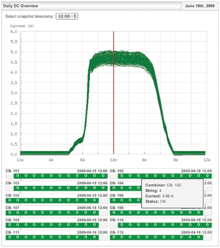
String Level Monitoring: (Figure 1, light green area) This is a way to get beyond the downside of simple array monitoring by narrowing the focus to individual strings of panels, eight to 18 modules in series. It is more expensive and complex, requiring special data acquisition equipment and a monitoring interface designed to interpret the data and render it into an understandable form, usually as a string graph spread over time. In return for the additional cost and complexity, the health of every string in the array becomes apparent (Figure 2). If one panel in a string of 12 fails or falls into shade, it will be apparent in string level monitoring and easy to locate within the array. Of course with more complexity comes a greater installation cost and more potential for component failure.

Several companies offer “smart” combiner boxes that measure and report string level currents. The technology is relatively inexpensive with the bulk of costs tied up in the installation of power and communications lines. The future may see reliable self-powered smart combiners with wireless communications that will significantly reduce installation costs and make retrofits simpler.

Micro Inverters: (Figure 1, dark green area). We placed an asterisk next to the micro inverter because it is a technology that changes the traditional SEF paradigm and is not yet proven over a full photovoltaic system lifespan. With micro inverters, the traditional array design–a central inverter fed by DC power collected from an array–is gone. Instead, a small inverter is attached to the back of every module in the array where it converts DC current directly into AC and sends it down a series line to combiners and ultimately to a production meter.

The system offers a plethora of advantages over traditional designs: AC wiring from inverter to inverter eliminates DC wire losses; DC current is measured at each module and the data is sent to a communications hub through the AC conductors eliminating the need for parallel communications lines; panel mismatch losses are eliminated and the loss of one panel will not affect output from neighboring panels. On the downside, the technology is more expensive than conventional DC inverters (even after eliminating DC wiring losses, communications wiring and panel mismatch losses). What’s more, it has precious little operating history, a factor that eliminates it from consideration by most financial institutions which back the construction of large solar electric facilities. While micro inverters could be the future industry standard, today’s focus on proven, long-term technology and lower costs will keep the use of traditional equipment and methods in place.

DC Power Conditioning: (Figure 1, dark green area) This technology offers benefits similar to micro inverters yet fits within the traditional SEF structure; again, a structure that is time proven and more easily funded. Like micro inverters, power conditioning units are mounted behind every panel in an array, wired in a string series, provide monitoring of individual module function, simplify array design and eliminate panel mismatch problems. But unlike micro inverters, the power conditioners do not invert DC to AC. Instead, they perform maximum power point tracking (MPPT) at the panel, lightening the MPPT load from the centralized inverter. The benefits are improved system efficiency and a more reliable inverter.

Currently, DC power conditioning adds more cost to a system than it saves, though this is expected to change relatively soon as the components are integrated into the panel junction box. Micro inverters may one day follow suit and perhaps by then they will be an accepted standard in solar finance.

System Size and Monitoring

Solar Power Partners works with some of the finest, most cautious finance institutions in the world. These relationships dictate that we build only the most reliable and predictable systems available. To that end, all of our SEFs are constructed with string level monitoring. It works well in our current market niche of 250kW to 2 MW arrays; yet, as we look ahead towards larger, utility scale projects, the economics of string level monitoring begin to suffer from diminishing returns.

For example, in a hypothetical 240kW system with 1,200 modules, the loss of one 12-module string can cause a noticeable 1 percent decrease in system production. That same string loss in a 5 MW project equates to a .048 percent decrease, a negligible loss that does not validate the cost of installing string level monitoring.

In these circumstances, we sacrifice granularity for the cost effectiveness of simple array monitoring while reducing the number of potential communications errors from the array. Improved granularity could soon return to large scale arrays once DC power conditioning becomes economically feasible. This is because the technology has the added benefit of providing array-wide, panel to panel communications either wirelessly or through the DC lines with little additional infrastructure.

Appropriate monitoring equipment, combined with accurate performance predictions, enables SPP to efficiently pursue two goals: optimize output and keep downtime to a minimum. We manage this on an ongoing basis through active monitoring and preventative maintenance.

Active Monitoring

It’s a rare breed of individual who can stare at a performance monitor through every daylight hour and not go a touch loopy. If humans were given this task, granularity of performance data would quickly become coarse. Thankfully, computers are quite adept at performing these tedious active-monitoring tasks with smart software that constantly monitors system performance and alerts the SEF manager to trouble through various alarms. This, however, does not completely remove the human from active monitoring.

Automated systems work well with absolutes: Is the inverter on? Is the communications system functioning? While important, these do little to help us audit system performance measured in degrees. To ensure a system is operating at optimal levels, the SEF manager establishes performance parameters within the monitoring system. However, these absolute parameters–defined as edges of acceptable system behavior–are created for a system operating in an environment with fluctuating edges, far from absolute. If the system strays outside the parameter limits, the automatic monitoring system raises an alarm to a possible problem but, because the system operates fluidly, ebbing and flowing with its environment, false alarms are the most likely result. To bypass this problem, the SEF manager will often set the operating parameters broadly, sacrificing accuracy and timeliness for peace and quiet.

In fact, this is the answer to effective monitoring with today’s systems. By allowing the computer to continuously scan for system faults and large production discrepancies, the SEF manager needs only to look for subtle performance changes at intermittent intervals. The frequency of interval will be defined by the amount of time available and the value of any gains in system efficiency made through human monitoring.

For example, if a slow moving cloud covers three strings of an array for 30 minutes, an alarm will not be issued because the system is programmed to wait two hours for the low strings to return to normal. If the string discrepancy does not clear out within the two-hour window, it is safe to assume our problem is not related to a static, rogue cloud and an alarm will be sent to the designated parties. In this case, we sacrifice the immediate knowledge of a possible fault in exchange for the time saved in ignoring a probable false alarm.

On the human side, we review our system string graphs (Figure 2, above) a few times a day looking for the obvious problems and perform a detailed assessment of production at the end of every month primarily to determine how soiling is affecting output. Monthly assessments are sufficient to track soiling as it pushes us towards our semi-scheduled preventative maintenance visits, the subject of Part II in the November/December issue.

Bryan Banke is director of Asset Management Services for Solar Power Partners and have been with the company since November 2007. He was a private solar PV project analyst and feasibility consultant with Banke Energy. His career in energy began in the 1980s as an analyst with Southwest Gas Corp.