An Overview of the U.S. Power Grid Model for the Geomagnetic Storm Threat Environments
The ability to comprehensively assess the vulnerability of the U.S. power grid to the
geomagnetic storm environment produced by solar activity stems from the parallel
investigations that have been underway to understand the problems of power system
vulnerability from high altitude nuclear-burst (HEMP) events. Power system impacts
from geomagnetic storms were first observed in 1940 and have been growing in
importance as the power system has grown over the intervening years.
Geomagnetic storms are created when the Earth's magnetic field captures ionized
particles carried by the solar wind due to coronal mass ejections or coronal holes at the
Sun. Although there are different types of disturbances noted at the Earth surface, the
disturbances can be characterized as a very slowly varying magnetic field, with rise times
as fast as a few seconds, and pulse widths of up to an hour. The rate of change of the
magnetic field is a major factor in creating electric fields in the Earth and thereby
inducing quasi-dc current flow in the power transmission network. Unlike the HEMP
threats, geomagnetic storms are a much more frequent occurrence, which also allows for
extensive opportunities to fully benchmark each component of the simulation models and
therefore provide greater confidence in the analysis of plausible severe threats, such as
the threat posed by an extreme geomagnetic storm scenario.
The context of the evolution of power system discoveries of vulnerability can be further
understood by an overview of the geomagnetic storm phenomena, which is closely
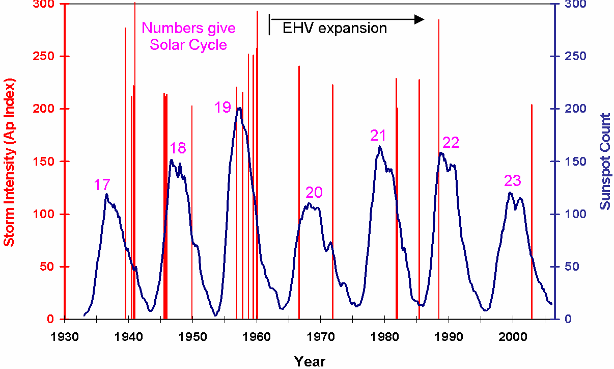
associated with the more familiar variability of the sunspot cycle. Figure 1-1 provides a
plot of the sunspot count as well as large geomagnetic storms over the last 70 years.
Because each sunspot cycle is typically ~11 years in duration, this plot provides the status
of the current solar cycle (Cycle 23) back to Cycle 17, which began in ~1932. As can be
seen, not all sunspot cycles are of equal intensity and Cycle 19 (late 1950’s-early 1960’s)
is in fact the largest sunspot cycle of human-record. The most recent cycle, Cycle 23,
exhibits a profile similar to that of Cycle 17. As noted in this figure, at the time of Cycle
19, much of the present U.S. power grid high-voltage transmission system of today did
not exist. To further explore the importance of the evolution of the power grid and its
growing vulnerability, it is necessary to look at specific large geomagnetic storms, as the
sunspot count does not provide sufficient correlations to impacts observed at the Earth.
In classification of the intensity of geomagnetic storms an index called the Ap index is
used, which provides a planetary measure of storm activity. Many of these storms caused
notable impacts to various terrestrial technology systems of their respective eras. The
storms of March 1989 and several in 1991 produced large and unprecedented operational
impacts to power grids in the U.S. and at other world locations. Also noteworthy is that
large geomagnetic storms generally have not occurred around the peaks of sunspot
activity. For example, a storm in February 1986 caused power system problems all
across the eastern U.S. but actually occurred at the absolute minimum between Solar
Cycle 21 and 22. Because sunspots only provide a gross measure of overall solar
activity, it does not accurately reflect the discrete eruptive events from violent solar
active regions that, when Earth-directed, can trigger large geomagnetic storms. Rather, it
is clear from this comparison that large and threatening geomagnetic storms can occur at
any time during the sunspot cycle, and pose a near continuous threat probability.
When reviewing the occurrence of large storms, it is important to recognize that the
problem of power system impacts is compounded by growing vulnerability of this
infrastructure to geomagnetic disturbances. The extent of the growth in vulnerability
over time is due to factors stemming from the growth of the high-voltage transmission
grid in the U.S., as well as changes within the grid that introduce new or enhance existing
impact problems to the power grid. Figure 1-2 shows the growth of the U.S. high voltage
transmission grid over the last 50 years. This geographically widespread infrastructure
readily couples through multiple ground points to the geo-electric field produced by
disturbances in the geomagnetic field. As shown, from Cycle 19 through Cycle 22, the
high voltage grid grew nearly tenfold. In essence, the antenna that is sensitive to
disturbances has grown dramatically over time. As this network has grown in size, it has
also grown in complexity. As will be discussed in later sections, one of the more
important changes in the technology base for the U.S. power grid that can increase
impacts to geomagnetic storms is the evolution to higher operating voltages of the
network. The operating levels of the high voltage network has increased from the 115-
230kV levels of the 1950’s to networks that operate from 345kV, 500kV and 765 kV
across the continent.
In order to quantify the impacts of the severe geomagnetic storm threats to the U.S.
power grid is it necessary to develop a series of models that translate the disturbed space
environment, or geomagnetic field environment, into specific impacts to the operation of
the electric power grid. This requires the following steps:
• Modeling in detail the geographically wide-spread disturbances to the
geomagnetic field from natural geomagnetic storm processes.
• Modeling the electromagnetic coupling between the disturbed space environment
and the deep-earth ground conductivity that produces a geo-electric field across
the surface of the Earth.
• Modeling the interaction between the geo-electric field and the complex power
grid topology to calculate the flow of geomagnetically induced current (GIC)
throughout the exposed power grid infrastructure.
• Modeling of the operational impacts in the U.S. power grid due to GIC flows
caused by either E3 threats or severe geomagnetic storm conditions.
While each of these models and associated environments are complex, these modeling
efforts have been highly successful in accurately replicating geomagnetic storm events
and performing detailed forensic analysis of geomagnetic storm impacts to electric power
systems. This capability has also been successfully applied towards providing predictive
geomagnetic storm forecasting services to the electric power industry. To further
describe the methodology used in this analysis, a brief overview is provided for each of
the key modeling steps that were undertaken.
An important facet of this investigation requires the simulation of geomagnetic storm
events and the impacts that these storms caused to electric power grid operation, and to
also investigate the potential impacts of very large storm events that have not recently
been experienced by today’s power systems. Electric power system operators realize that
large and severe geomagnetic storms (such as the March 1989 storm) have the potential
to cause important power system impacts. However, the U.S. power industry in general
have not developed comprehensive simulation models such as being developed in this
effort to better quantify the nature of the threat environment. The power industry also has
a very limited perspective on the extremes of storm intensity due to the flaws of the K
Index rating of storms. While some past storms have severely threatened the U.S. grid,
these storms do not represent the most severe storm events that are plausible. Therefore,
comprehensive models allow the development of improved understandings of the
extremes of the geomagnetic environment and consequential impacts that future severe
storms may pose to the integrity of this important infrastructure...
Geomagnetic disturbances are caused by interactions of the solar wind with the Earth’s
magnetic field. There are a number of ways that a geomagnetic storm can produce a
ground-level geomagnetic field disturbance that could have the potential to impact power
system operations. One of the most important geomagnetic storm processes involves the
intensification and flow of ionospheric currents known as electrojets. These electrojets
are formed around the north and south magnetic poles at altitudes of about 100km and
can have magnitudes of ~1 million amps, which is sufficient in intensity to cause widespread
disturbances to the geomagnetic field. Because of the large geographic scale of
the U.S. power grid, it would not be suitable to assume the application of a simple planewave
model for the disturbance conditions. Therefore, to simulate the geomagnetic storm
environment, it is necessary to develop a geographically gridded specification of the
complex spatial and temporal dynamics of the disturbances as they propagate across
North American locations that are to be modeled....
Figure 1-3 shows the vector description of a disturbance of the geomagnetic
field simultaneously observed at a number of locations across North America at time 9:10
UT May 10, 1992.

...Ground conductivity models need to accurately reproduce geo-electric field variations
that are caused by the very low frequency ranges of geomagnetic storms. These
electromagnetic disturbances require models accurate over a frequency range from 0.3 Hz
to as low as 0.00001 Hz. Because of the low-frequency content of the disturbance
environments, it is necessary to take into consideration ground conductivities to
appropriate depths...
These conductivity variations with depth can range 3 to 5 orders of
magnitude. While surface conductivity can exhibit considerable lateral heterogeneity
across the U.S., conductivity at depth is more uniform. Because of this, models of ground
conductivity can be successfully applied over meso-scale distances and can be accurately
represented by use of layered conductivity profiles or models. Frequent occurrences of
geomagnetic storm events and subsequent measurement of these storm environments and
associated impacts have provided opportunities to use this information to develop and
validate models of the ground conductivity for the U.S. Power Grid Model.
A severe electrojet disturbance can produce a rate-of-change intensity profile (or dB/dt)
of 2400 nT/min or greater. This disturbance is a very severe disturbance that could be
possible at high to mid latitude locations throughout the U.S...
a map of the overall transmission network included in the CONUS
region model of the U.S. grid. The major transmission voltages are color highlighted by
operating voltage with the three operating voltages of 345kV, 500kV and 765kV (there
are also several lines in the Washington state region that are operated at 300kV which are
included in the model, and in the figure are combined with 345kV lines). Figure 1-10
provides the mileage statistics for each of these three voltage classes that are represented
in the U.S. model for the CONUS region. As shown, the most common transmission
voltage is the 345kV, which makes up about 64% of total transmission line miles. The
highest operating voltage is the 765kV and is primarily located in the Illinois, Ohio,
Indiana, West Virginia and upstate New York regions of the U.S. Both the 345kV and
500kV portions of the network are more widely distributed across the U.S...

Figure 1-9. Map of 345kV, 500kV and 765kV substations and transmission network in U.S. grid model.
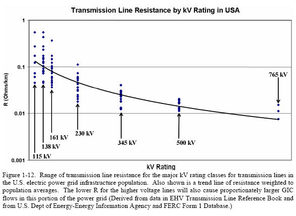
The operating voltage of the transmission network is an important factor in determining
the level of GIC flow that will occur on each part of the U.S. power grid. At the higher
operating voltages, there are pronounced trends that: the average length of each line
increases and the average circuit resistance decreases. These trends result in larger GIC
flows in the higher voltage portions of the network, given the same geo-electric field
conditions...
Transformers also exhibit a general characteristic of lower resistance as kV rating
increases. However, the trend in transformer design is even more pronounced as a
function of MVA or current rating of the transformer. It is generally consistent that the
higher MVA rated transformers are also the highest kV rated transformers, though there
can be a few exceptions.
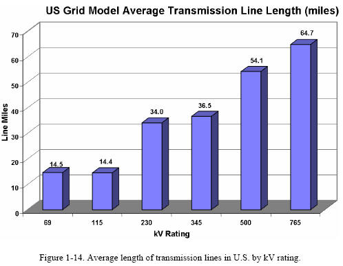
In addition to the lower resistances at the higher kV rating lines on the network, average
length of these lines also introduces a higher overall risk of GIC flows as well. Figure 1-
14 provides a summary of average transmission line lengths in the U.S. by kV rating. As
illustrated, the average length of transmission lines also increases significantly with
increased kV ratings. The 765kV lines average over 60 miles in length while the 115kV
lines are less than 15 miles in average length. While predicting GIC flows, it is necessary
to take into consideration the network topology as a integrated whole. It is evident that
on an individual line basis a combination of longer average length (and increased geoelectric
potential between end points of the line) combined with lower average resistances
will produce substantially larger GICs on average in the higher voltage portions of the
power grid.